QM/MM Protocol for Direct Molecular Dynamics of Chemical Reactions in Solution: The Water-Accelerated Diels–Alder Reaction

Yang, Z.; Doubleday, C.; Houk, K. N. J. Chem. Theor. Comput. 2015,  5606-5612
Contributed by Steven Bachrach
Reposted from Computational Organic Chemistry with permission

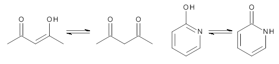
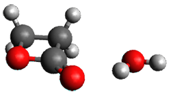
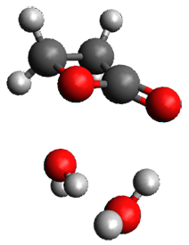
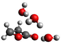
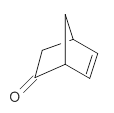
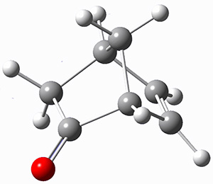
I discuss the aqueous Diels-Alder reaction in Chapter 7.1 of my book. A key case is the reaction of methyl vinyl ketone with cyclopentadiene, Reaction 1. The reaction is accelerated by a factor of 740 in water over the rate in isooctane.¹ Jorgensen argues that this acceleration is due to stronger hydrogen bonding to the ketone than in the transition state than in the reactants.^2-4

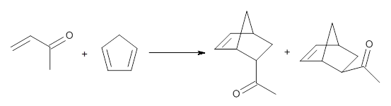
Rxn 1

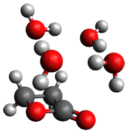
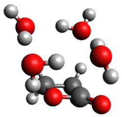
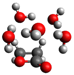
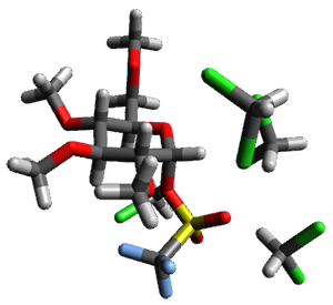
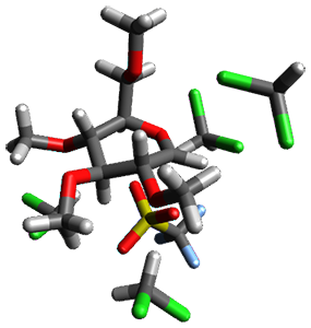
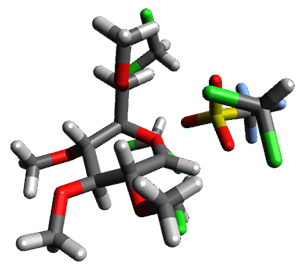
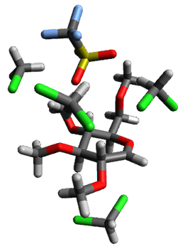
Doubleday and Houk⁵ report a procedure for calculating trajectories including explicit water as the solvent and apply it to Reaction 1. Their process is as follows:

1. Compute the endo TS at M06-2X/6-31G(d) with a continuum solvent.
2. Equilibrate water for 200ps, defined by the TIP3P model, in a periodic box, with the transition state frozen.
3. Continue the equilibration as in Step 2, and save the coordinates of the water molecules after every addition 5 ps, for a total of typically 25 steps.
4. For each of these solvent configurations, perform an ONIOM computation, keeping the waters fixed and finding a new optimum TS. Call these solvent-perturbed transition states (SPTS).
5. Generate about 10 initial conditions using quasiclassical TS mode sampling for each SPTS.
6. Now for each the initial conditions for each of these SPTSs, run the trajectories in the forward and backward directions, typically about 10 of them, using ONIOM to compute energies and gradients.
7. A few SPTS are also selected and water molecules that are either directly hydrogen bonded to the ketone, or one neighbor away are also included in the QM portion of the ONIOM, and trajectories computed for these select sets.

The trajectory computations confirm the role of hydrogen bonding in stabilizing the TS preferentially over the reactants. Additionally, the trajectories show an increasing asynchronous reactions as the number of explicit water molecules are included in the QM part of the calculation. Despite an increasing time gap between the formation of the first and second C-C bonds, the overwhelming majority of the trajectories indicate a concerted reaction.

References

(1) Breslow, R.; Guo, T. "Diels-Alder reactions in nonaqueous polar solvents. Kinetic
effects of chaotropic and antichaotropic agents and of β-cyclodextrin," J. Am. Chem. Soc. 1988, 110, 5613-5617, DOI: 10.1021/ja00225a003.

(2) Blake, J. F.; Lim, D.; Jorgensen, W. L. "Enhanced Hydrogen Bonding of Water to Diels-Alder Transition States. Ab Initio Evidence," J. Org. Chem. 1994, 59, 803-805, DOI: 10.1021/jo00083a021.

(3) Chandrasekhar, J.; Shariffskul, S.; Jorgensen, W. L. "QM/MM Simulations for Diels-Alder
Reactions in Water: Contribution of Enhanced Hydrogen Bonding at the Transition State to the Solvent Effect," J. Phys. Chem. B 2002, 106, 8078-8085, DOI: 10.1021/jp020326p.

(4) Acevedo, O.; Jorgensen, W. L. "Understanding Rate Accelerations for Diels−Alder Reactions in Solution Using Enhanced QM/MM Methodology," J. Chem. Theor. Comput. 2007, 3, 1412-1419, DOI:10.1021/ct700078b.

(5) Yang, Z.; Doubleday, C.; Houk, K. N. "QM/MM Protocol for Direct Molecular Dynamics of Chemical Reactions in Solution: The Water-Accelerated Diels–Alder Reaction," J. Chem. Theor. Comput. 2015, , 5606-5612, DOI: 10.1021/acs.jctc.5b01029.

This work is licensed under a Creative Commons Attribution-NoDerivs 3.0 Unported License.

A Local Variant of the Conductor-Like Screening Model for Fragment-Based Electronic-Structure Methods

Albrecht Goez and Johannes Neugebauer J. Chem. Theory Comput., Article ASAP, DOI: 10.1021/acs.jctc.5b00832
Contributed by Christoph Jacob
 
Fragment-based methods nowadays make it possible to perform quantum-chemical calculations for rather large biomolecules, for instance light-harvesting protein systems [1]. Such methods are based on the idea of splitting a protein into smaller fragments, such as its constituting amino acids. This leads to a linear scaling of the computational effort with the size of protein. Popular examples of fragment-based electronic structure methods include the fragment molecular orbital (FMO) method [2] and a generalization of the frozen-density embedding scheme (3-FDE) [3].

In a recent article in JCTC, Goez and Neugebauer from the University of Münster (Germany) address an additional bottleneck that appears in such calculations. Usually, it is necessary to include a solvent environment in the calculations, in particular if charged amino-acid side chains are present. The simplest way of doing so are continuum solvation models, such as COSMO or PCM. These models represent the solvent in terms of apparent charges on the surface of a cavity enclosing the protein. However, for proteins the number of apparent surfaces charges becomes rather large - for ubiquitin, a protein with only 78 amino acids, already 20,000 charges are needed. Updating these apparent surface charges involves solving a linear system of equations of size 20,000 x 20,000. When doing so in each SCF cycle for each of the fragments, the continuum solvation model will become the bottleneck of the calculation.

To solve this problem, Goez and Neugebauer developed a local variant of the COSMO model (LocCOSMO). In each fragment calculation, they update only those apparent surface charges that are close to this fragment. This reduces the computational effort significantly, but because every fragment is updated at some point it will eventually result in the same final result. This is demonstrated by the authors for several test cases. They can reduce the computational time required for a 3-FDE calculation of ubiquitin in a solvent environment by a factor of 30, without compromising the quality of the result.

The efficient combination of fragment-based quantum chemistry with continuum solvation models  provides an important tool for studies of biomolecules. It will make such calculations more robust by alleviating convergence problems for charged amino acids and will allow for a more realistic inclusion of protein environments in studies of spectroscopic properties of chromophores in biomolecular systems.

References:

[1] A. Goez, Ch. R. Jacob, J. Neugebauer, “Modeling environment effects on pigment site energies: Frozen density embedding with fully quantum-chemical protein densities”, Comput. Theor. Chem. 1040–1041, 347–359 (2014).
[2] D. G. Fedorov, K. Kitaura, “Extending the Power of Quantum Chemistry to Large Systems with the Fragment Molecular Orbital Method”, J. Phys. Chem. A 111, 6904–6914 (2007).
[3] Ch. R. Jacob, L. Visscher, “A subsystem density-functional theory approach for the quantum chemical treatment of proteins”, J. Chem. Phys. 128, 155102 (2008).

Benchmarking Continuum Solvent Models for Keto–Enol Tautomerizations

McCann, B. W.; McFarland, S.; Acevedo, O. J. Phys. Chem. A 2015, 119, 8724-8733
Contributed by Steven Bachrach.
Reposted from Computational Organic Chemistry with permission

The keto-enol tautomerization is a fundamental concept in organic chemistry, taught in the introductory college course. As such, it provides an excellent test reaction to benchmark the performance computational methods. Acevedo and colleagues have reported just such a benchmark study.¹

First, the compare a wide variety of methods, ranging from semi-empirical, to DFT, and to composite procedures, with experimental gas-phase free energy of tautomerization. They use seven such examples, two of which are shown in Scheme 1. The best results from each computation category are AM1, with a mean absolute error (MAE) of 1.73 kcal mol^-1, M06/6-31+G(d,p), with a MAE of 0.71 kcal mol^-1, and G4, with a MAE of 0.95 kcal mol^-1. All of the modern functionals do a fairly good job, with MAEs less than 1.3 kcal mol^-1.

Scheme 1

As might be expected, the errors were appreciably larger for predicting the free energy of tautomerization, with a good spread of errors depending on the method for handling solvent (PCM, CPCM, SMD) and the choice of cavity radius. The best results were with the G4/PCM/UA0 procedure, though M06/6-31+G(d,p)/PCM and either UA0 or UFF performed quite well, at considerably less computational expense.

References

(1) McCann, B. W.; McFarland, S.; Acevedo, O. "Benchmarking Continuum Solvent Models for Keto–Enol Tautomerizations," J. Phys. Chem. A 2015, 119, 8724-8733, DOI: 10.1021/acs.jpca.5b04116.

This work is licensed under a Creative Commons Attribution-NoDerivs 3.0 Unported License.

Water–Water and Water–Solute Interactions in Microsolvated Organic Complexes

Pérez, C.; Neill, J. L.; Muckle, M. T.; Zaleski, D. P.; Peña, I.; Lopez, J. C.; Alonso, J. L.; Pate, B. H. Angew. Chem. Int. Ed. 2015, 54, 979-982
Contributed by Steven Bachrach.
Reposted from Computational Organic Chemistry with permission

The structure of water about a solute remains of critical importance towards understanding aqueous solvation. Microwave spectroscopy and computations are the best tools we have today to gain insight on this problem. This is nicely demonstrated in the Alonso study of the microsolvated structures of β-propiolactone 1.¹ They employed chirped-pulse Fourier transform microwave (CP-FTMW) spectroscopy and MP2(fc)/6-311++G(d,p) computations to examine the structure involving 1-5 water molecules.

The computed structures of these microsolvated species are shown in Figure 1. The deviation of the computed and experimental structures (RMS in the atomic positions) is small, though increasing as the size of the cluster increases. The deviation is 0.014 Å for the 1^. H₂O cluster and 0.244 Å for the 1^.(H₂O)₅cluster. They identified two clusters with four water molecules; the lower energy structure, labeled as a, is only 0.2 kJ mol^-1 more stable than structure b.

1.H2O	1.(H2O)2
1.(H2O)3
1.(H2O)4 a	1.(H2O)4 b
1.(H2O)5

Figure 1. MP2(fc)/6-311++G(d,p) optimized geometries of the hydrates of 1.

Water rings are found in the clusters having four or five water molecules, while chains are identified in the smaller clusters. One might imagine water cages appearing with even more water molecules in the microsolvated structures.

References

(1) Pérez, C.; Neill, J. L.; Muckle, M. T.; Zaleski, D. P.; Peña, I.; Lopez, J. C.; Alonso, J. L.; Pate, B. H. Angew. Chem. Int. Ed. 2015, 54, 979-982, DOI: 10.1002/anie.201409057.

InChIs

1: InChI=1S/C3H4O2/c4-3-1-2-5-3/h1-2H2
InChIKey=VEZXCJBBBCKRPI-UHFFFAOYSA-N

This work is licensed under a Creative Commons Attribution-NoDerivs 3.0 Unported License.

Theoretical Foundation for the Presence of Oxacarbenium Ions in Chemical Glycoside Synthesis

Hosoya, T.; Takano, T.; Kosma, P.; Rosenau, T.  J. Org. Chem. 2014, 79, 7889-7894

Contributed by Steven Bachrach.
Reposted from Computational Organic Chemistry with permission

Comparing S_N2 and S_N1 reactions using computational methods is often quite difficult. The problem is that the heterolytic cleavage in the S_N1 reaction leads to an ion pair, and in the gas phase this is a highly endothermic process. Optimization of the ion pair in the gas phase invariably leads to recombination. This is disturbingly the result even when one uses PCM to mimic the solvent, which one might have hoped would be sufficient to stabilize the ions.

The computational study of the glycoside cleavage by Hosoya and colleagues offers some guidance towards dealing with this problem.¹ They examined the cleavage of triflate from 2,3,4,6-tetra-O-methyl-α-D-glucopyranosyl triflate 1.

Benchmarking the dissociation energy for the cleavage of 1 and considering computational performance, they settled on M06-2X/BS-III//M06-2X/BS-I, where BS-III is aug-cc-pVTZ basis set for O, F, and Cl and cc-pVTZ for H, C, and S and BS-I is 6-31G(d,p) basis sets were employed for H, C, and S, and 6-31+G(d) for O, F, and Cl. Solvent (dichloromethane) was included through PCM.

Attempted optimization of the contact ion pair formed from cleavage of 1 invariably led back to the covalent bound 1. PCM is not capable of properly stabilizing these types of ions in proximity. To solve this problem, they incorporated four explicit dichloromethane molecules. A minor drawback to their approach is that they did not sample much of configuration space and so their best geometries may not be the lowest energy configurations. Nonetheless, with four solvent molecules, they were able to locate contact ion pairs and solvent-separated ion pairs. Representative examples are shown in Figure 1. This method of explicit incorporation of a few solvent molecules seems to be the direction we must take to treat ions or even highly polar molecules in solution.

1 0.0	1-CIP 8.5
1-SSIPa 8.4	1-SSIPb 11.1

Figure 1. Representative examples of microsolvated 1, its contact ion pair (CIP) and solvent separated ion pair (SSIP) computed at M06-2X/BS-III//M06-2X/BS-I, and relative energies (kcal mol^-1)

References

(1) Hosoya, T.; Takano, T.; Kosma, P.; Rosenau, T. "Theoretical Foundation for the Presence of Oxacarbenium Ions in Chemical Glycoside Synthesis," J. Org. Chem. 2014, 79, 7889-7894, DOI:10.1021/jo501012s.

InChIs

1: InChI=1S/C11H19F3O8S/c1-17-5-6-7(18-2)8(19-3)9(20-4)10(21-6)22-23(15,16)11(12,13)14/h6-10H,5H2,1-4H3/t6-,7-,8+,9-,10-/m1/s1
InChIKey=RPZNYYCDDYUPJR-HOTMZDKISA-N

Update: be sure to read the interesting discussion associated with this post on Computational Organic Chemistry.


This work is licensed under a Creative Commons Attribution-NoDerivs 3.0 Unported License.

Large Solvation Effect in the Optical Rotatory Dispersion of Norbornenone

Lahiri, P.; Wiberg, K. B.; Vaccaro, P. H.; Caricato, M.; Crawford, T. D. Angew. Chem. Int. Ed. 2014, 53, 1386
Contributed by Steven Bachrach.
Reposted from Computational Organic Chemistry with permission

Optical activity is a major tool for identifying enantiomers. With recent developments in computational techniques, it is hoped that experiments combined with computations will be a powerful tool for determining absolute configuration. The recent work of Lahiri, et al. demonstrates the scope of theoretical work that is still needed to really make this approach broadly applicable.¹

They prepared (1R,4R)-norbornenone 1 and measured its optical rotation in the gas phase and in dilute solutions of acetonitrile and cyclohexane. The specific rotations at three different wavelengths are listed in Table 1. Of first note is that though there is some small differences in solution, as expected, there really is substantial differences between the gas- and solution phases. Thus cautionary point 1: be very careful of comparing solution phase experimental optical activity with computed gas phase predictions.

1

Table 1. Experimental and computed specific rotation of 1.

	355.0 nm	589.3 nm	633.0 nm
Gas phase
Expt	6310	755	617
B3LYP	10887	1159	944
CCSD	3716	550	453
Acetonitrile solution
Expt	8607	950	776
PCM/B3LYP	11742	1277	1040
Cyclohexane solution
Expt	9159	981	799
PCM/B3LYP	11953	1311	1069

For the computations, the geometry of 1 was optimized at B3LYP/aug-cc-pVTZ (see Figure 1. The OR was computed at B3LYP with different basis sets, finding that the difference in the predicted specific rotation at 598.3nm differs only quite little (90.6 deg dm^-1 (g/mL)^-1) between the computations using aug-cc-pVTZ and aug-cc-pVQZ) suggesting that the basis set limit has been reached. The gas –phase computed values at B3LYP and CCSD are also shown in Table 1. Though these computations do get the correct sign of the rotation, they are appreciably off of the experimental values, and the percent error varies with wavelength. Cautionary point 2: it is not obvious what is the appropriate computational method to compute OR, and beware of values that seem reasonable at one wavelength – this does not predict a good agreement at a different wavelength.

Figure 1. Optimized geometry of 1 at B3LYP/aug-cc-pVTZ.

Lastly, computed solution values of the OR were performed with PCM and B3LYP. These values are given in Table 1. Again the agreement is poor. So cautionary point 3: computed (PCM) solution OR
may be in quite poor agreement with experiment.

Often the culprit to poor agreement between computed and experimental OR is attributed to omitted vibrational effects, but in this case, because 1 is so rigid, one might not expect too much error to be caused by the effects of vibrations. So the overall result – we need considerable work towards addressing how to accurately compute optical activity!

References

(1) Lahiri, P.; Wiberg, K. B.; Vaccaro, P. H.; Caricato, M.; Crawford, T. D. "Large Solvation Effect in the Optical Rotatory Dispersion of Norbornenone," Angew. Chem. Int. Ed. 2014, 53, 1386-1389, DOI:10.1002/anie.201306339.

InChIs

1: InChI=1S/C7H8O/c8-7-4-5-1-2-6(7)3-5/h1-2,5-6H,3-4H2/t5-,6+/m1/s1
InChIKey=HUQXEIFQYCVOPD-RITPCOANSA-N

This work is licensed under a Creative Commons Attribution-NoDerivs 3.0 Unported License.

The Binding of Benzoarylsulfonamide Ligands to Human Carbonic Anhydrase is Insensitive to Formal Fluorination of the Ligand

Matthew R. Lockett, Heiko Lange, Benjamin Breiten, Annie Heroux, Woody Sherman, Dmitrij Rappoport, Patricia O. Yau, Philip W. Snyder, and George M. Whitesides Angew. Chem. Int. Ed. 2013, 52, 7714
Contributed by +Jan Jensen

Accurate modeling the hydrophobic effect (or effects) is probably the biggest challenge to computational drug design (see for example this CC Highlight).  The hydrophobic effect on protein-ligand binding is generally thought to come from the release of structured and entropically unfavorable water molecules from the hydrophobic surfaces of the ligand and binding pocket. However, is also possible that the release of strongly bound water molecules to the protein/or ligand contributes to this effect.

I find this article important for two reasons:

1) The thorough characterization, including x-ray structures, of the binding of homologous ligands provides a valuable benchmark for computational studies.  The authors show that fluorination, commonly thought to increase the hydrophobic contribution to the binding free energy indeed increases the entropy of binding, but does so without decreasing the binding free energy.

The fluorinated ligand is indeed more hydrophobic as measured by buffer/octanol partitioning so what's going on?  One answer may be the difference in strongly bound water molecules observed in the protein-ligand x-ray structures: six and ten for the un- and fluorinated ligand, respectively. However, a simple correction based on the number of strongly bound water molecules is unlikely: a homologous un- and fluorinated ligand pair showed large differences in the binding enthalpy and entropy but smaller difference in number of strongly bound water molecules (four and seven, respectibely).

2) The supplementary material provides a fantastic list of important papers in this area.  I have reproduced the list below and added links, where available, to the articles.

From supplementary materials

Water-centric view of protein-ligand binding (relevant references in chronological order).

1. Solvation. A Molecular Dynamics Study of a Dipeptide in Water. 

2. A Direct Measure of the Contribution of Solvent Reorganization to the Enthalpy of Binding.

3. How Water Provides the Impetus for Molecular Recognition in Aqueous Solution. 

4. Thermodynamic Solvent Isotope Effects and Molecular Hydrophobicity, Adv. Biophys. Chem. 1997, 6, 1 (not available on-line)

5. Hydrophobicity at Small and Large Length Scales. 

6. Computational Prediction of Native Protein Ligand-Binding and Enzyme Active Site Sequences.

7. Role of the Active-Site Solvent in the Thermodynamics of Factor Xa Ligand Binding. 

8. Hydrophobicity of Protein Surfaces: Separating Geometry from Chemistry.

9. The Thermodynamics of Protein-Ligand Interaction and Solvation: Insights for Ligand Design.

10. Dewetting and Hydrophobic Interactions in Physical and Biological Systems.

11. Extent of Enthalpy-Entropy Compensation in Protein-Ligand Binding.

12. Contribution of Explicit Solvent Effects to the Binding Affinity of Small-Molecule Inhibitors in Blood Coagulation Factor Serine Proteases.

13. Dissecting the Hydrophobic Effect on the Molecular Level: the Role of Water, Enthalpy, and Entropy in Ligand Binding to Thermolysin.

14. Ligand Binding Stepwise Disrupts Water Network in Thrombin: Enthalpic and Entropic Changes Reveal Classical Hydrophobic Effect.

15. Development of New Cyclic Plasmin Inhibitors with Excellent Potency and Selectivity.

Enthalpy-entropy compensation in protein-ligand binding (relevant references in chronological order).

1. Enthalpy-Entropy Compensation Phenomena in Water Solutions of Proteins and Small Molecules: A Ubiquitous Propery of Water.

2. Win Some, Lose Some—Enthalpy-Entropy Compensation in Weak Intermolecular Forces. (pdf)

3. Application of a Generalized Enthalpy-Entropy Relationship to Binding Cooperativity and Weak Associations in Solution.

4. Enthalpy-Entropy Compensation is not a General Feature of Weak Association. 

5. Extent of Enthalpy-Entropy Compensation in Protein-Ligand Binding.

6. Thermodynamics of Ligand Binding and Efficiency.

7. A Multidisciplinary Approach to Probing Enthalpy-Entropy Compensation and the Interfacial Mobility Model.

8. Enthalpy-Entropy Transduction Caused by Conformational Shifts can Obscure the Forces Driving Protein-Ligand Binding.

9. Extreme Entropy-Enthalpy Compensation in a Drug-Resistant Variant of HIV-1 Protease.

10. Dissecting the Hydrophobic Effect on the Molecular Level: the Role of Water, Enthalpy, and Entropy in Ligand Binding to Thermolysin.

I thank Derek Lowe for bringing this paper to my attention

This work is licensed under a Creative Commons Attribution 3.0 Unported License.

Supramolecular Binding Thermodynamics by Dispersion-Corrected Density Functional Theory

Stefan Grimme Chemistry A European Journal 2012, 18, 9955 (Paywall)
Contributed by +Jan Jensen

Computing accurate binding free energies is a fundamental challenge to molecular modeling.  I recently highlighted a study by +Hari Muddana and +Michael Gilson where the binding free energies of 29 ligands to the host CB7 were reproduced with an RMSE of 1.9 kcal/mol using  PM6-DH+, though this involved fitting of the solvation free energy change.

In this study Grimme presents a computational methodology that reproduces binding free energies of 13 chemically diverse host-guest complexes with a MAD of 2.1 kcal/mol.  Though the accuracies of the two studies are similar there are many differences between the two approaches.

The gas phase interaction energies are computed using dispersion corrected DFT calculations.  Practically, this means that, unlike the study by Muddana and Gilson, no conformational averaging is performed.  The dispersion correction includes a three-body term that is shown to contribute up to 4.6 kcal/mol to the gas phase interaction energy.  The similar three-body terms also contribute to the vibrational free energy contributions (see below) and together with the gas phase contributions lower the MAD by 1.3 kcal/mol compared to experimental binding free energies.

Similarly, the solvation free energy is computed using DFT and COSMO and, unlike the Muddana and Gilson paper, is not corrected empirically.  This may be due to the fact that the DFT/COSMO calculations (including the radii used to define the surface) already has been carefully calibrated while the PM6/COSMO calculations have not.

The vibrational free energy corrections are computed in the gas phase using dispersion and hydrogen-bond corrected PM6 and DFTB (PM6-D3H and DFTB-D3H, respectively).  These corrections were developed as part of this study based on the S66 data set and implemented in an external program interfaced with the MOPAC and DFTB codes (Grimme, personal communications).

The vibrational entropy contribution increases exponentially with decreasing vibrational frequency and this can introduce numerical unstable binding free energies for these systems as low vibrational frequencies are common.  Grimme deals with this problem by introducing a hybrid function where the vibrational entropy is smoothly replaced (using a switching function) with a corresponding free-rotor entropy for low frequency modes.  As computed in his study, the free-rotor entropy increases much less steeply as the vibrational frequency decreases and produced binding free energies that are in better agreement with experiment. However, computing numerically stable vibrational frequencies for low frequency modes remains a challenge for these systems and may require manual intervention (Grimme, personal communications).  

Thanks to +Hari Muddana for alerting me to this paper and to Stefan Grimme for personal communications.

 
This work is licensed under a Creative Commons Attribution 3.0 Unported License. 

FixSol solvation model and FIXPVA2 tessellation scheme

Nandun M. Thellamurege and Hui Li Journal of Chemical Physics 2012 137, 246101 (Paywall)

Contributed by Jan H. Jensen

This paper introduces a variant of the conductor like polarizable continuum model (C-PCM) called FixSol and a modified area tesselation scheme (FIXPVA2) that both serve to increase the numerical stability of geometry optimizations and molecular dynamics simulations.

The C-PCM equation is $${\bf Cq}=-\frac{\varepsilon-1}{\varepsilon}{\bf V}\text{ where } C_{ij}=\frac{1}{r_{ij}}$$Here $r_{ij}$ is the distance between tesserae centers so when atomic spheres and, hence, tesserae points get close the C-PCM equations become numerically unstable.

This has traditionally been dealt with by associating damping functions with each tesserae point (see for example the work by York and Karplus) and FIXPVA2 is a variant of this approach.  However, this study goes even further and modified the $C$ matrix for tesserae that are within a certain cutoff with a smooth transition to C-PCM beyond the cutoff.  The resulting energies are within 0.5 kcal/mol of conventional C-PCM calculations for small molecule ab initio calculations.

However, what really caught my eye was that the demonstration of numerical stability was done by short (10-ps) FixSol-PCM/CHARMM molecular dynamics simulations of a small protein and 13-base pair piece of DNA with energy conservation to within 0.09 kcal/mol.  This is indeed a very stringent text of numerical stability and I don't recall having seeing PCM MD simulations on such large systems, but feel free to correct me in the comments.  Unfortunately timings where not given.

Full disclosure: I was Hui Li's PhD advisor


This work is licensed under a Creative Commons Attribution 3.0 Unported License. 

Calculation of Host-Guest Binding Affinities Using a Quantum-Mechanical Energy Model

Hari S. Muddana and Michael K. Gilson J. Chem. Theory Comput. 2012, 8, 2023 (Paywall)

Contributed by Jan Jensen

This paper presents absolute binding energies for 29 ligands complexed with cucurbit[7]uril (CB7) computed using PM6-DH+ and the COSMO solvation model.  

This is a great model system for studying binding: CB7 is a macrocyclic molecule made of seven fused-ring monomers and has only one conformational minimum.  Many of the 29 ligands for which binding free energies have been measure experimentally are also conformationally restricted, and the binding free energies span a wide range: -5.3 to -21.5 kcal/mol. 

Because of this a fairly exhaustive conformational search was feasible and the number of conformations per complex ranged from 5 to 300 depending on the flexibility of the guest.  The conformational search was done using the OPLS-2005 all-atom force field and a low-mode conformational search algorithm implemented in the Schrodinger software suite. 

These structures where then used as a starting point for PM6-DH+/COSMO energy minimizations and subsequent vibrational analysis.  Given the number of conformations and ligands this paper represents a significant investment of CPU time even at a semiempirical level of theory.  The COSMO solvation energy is augmented by a non-polar solvation term that depends on the molecular surface area.  Though not explicitly stated this must have been done as a single point correction.

The computed binding energies correlate well ($R^2$=0.79) with the experimental results, but the root-mean-square error (RMSE) is high (11.4 kcal/mol) suggesting a systematic error.  To address this a three parameter fit was made involving the COSMO and non-polar solvation energy plus an off-set, which led to a $R^2$=0.91 and RMSE of 1.9 kcal/mol, excluding one outlier.  This analysis suggests that the COSMO solvation energies are overestimated by 4%, consistent with a similar analysis performed on 367 solvation energies for small neutral molecules.

The off-set was found to be -5.83 kcal/mol, i.e. the predicted binding energies are systematically underestimated by nearly 6 kcal/mol.  Interestingly, a recent analysis of explicit solvation thermodynamics of CB7, by Gilson and co-workers, "suggests that the water molecules in the CB7 cavity are unstable relative to bulk ...  If so, then treating the water in the cavity as a bulk dielectric might lead to a significant overestimation of the host’s solvation free energy and hence the underestimations of binding affinities observed here."  Furthermore, very recently  Rogers et al. was able to compute an absolute binding energy for one of the ligands to CB7 using thermodynamic integration and explicit solvent that was in excellent agreement with experiment.

The paper also provides a useful outline of how the thermodynamical aspects should be handled and analyzed, including a nice analysis of the conformational entropy change.  For example, the translational entropy must be computed using a volume of 1 L rather than that of an ideal gas a 1 bar, and that one should compute the Helmholtz, rather than the Gibbs, free energy change since the change in volume of the solution upon binding is negligible in the condensed phase.  There is also a reference to a real gem of a paper by Zhou and Gilson that reconciles the rigid rotor-harmonic oscillator approach to thermodynamics used here with that used in molecular dynamics studies.

While the agreement with experiment is impressive there is some room for improvement and this system provides a great model system for testing all aspects of the binding energy including ab initio calculations of the interaction energy and new continuum solvation methods.

This work is licensed under a Creative Commons Attribution 3.0 Unported License. 

Variational approach for nonpolar solvation analysis

Zhan Chen, Shan Zhao, Jaehun Chun, Dennis G. Thomas, Nathan A. Baker, Peter W. Bates, and G. W. Wei Journal of Chemical Physics 2012, 137, 084101 (Paywall)

As I discussed in a previous highlight, work by Ryde and co-workers suggest that one of the main obstacles to predicting accurate protein-ligand binding constants using continuum solvation models is the non-polar contributions to the change solvation energy. 

I was therefore intrigued when ResearchGate alerted me to a new publication co-authored by Nathan Baker on a variational approach to non-polar solvation.  In this approach the solute-solvent boundary surface is varied to minimize the non-polar solvation energy.  The non-polar solvation energy is a function of the area and volume of the boundary surface and the solute-solvent van der Waals interactions.  

The current implementation of the method contains three adjustable parameters: the surface tension and hydrodynamic pressure of the solvent and the well-depth of the Lennard-Jones potential describing the solute-solvent interaction.  These parameters were obtained by fitting to experimental solvation energies of 11 alkanes, with an RMSD of 0.12 kcal/mol.  These parameters were then used to predict the solvation energy of 19 new alkanes, with a resulting RMSD of 0.31 kcal/mol.  The solvation energies of the 11 alkanes used for calibration are shown to be significantly more accurate than those obtained by explicit solvation. 

It will be very interesting to see whether this approach will lead to significantly better protein-ligand binding energies, but several issues will have to be addressed first: How will the be necessary parameters be obtained?  Is the approach efficient enough to handle protein-sized systems?  Does the variationally determined solute-solvent surface lead to good polar solvation energies?  It will be interesting to find out.

This work is licensed under a Creative Commons Attribution 3.0 Unported License.  

Accurate Predictions of Nonpolar Solvation Free Energies Require Explicit Consideration of Binding-Site Hydration

Samuel Genheden, Paulius Mikulskis, LiHong Hu, Jacob Kongsted, Pär Söderhjelm, and Ulf Ryde Journal of the American Chemical Society 2011, 133, 13092 (Paywall)

ab initio prediction of protein-ligand binding free energies

Fast computers and clever algorithms have made it possible to calculate protein-ligand binding energies ab initio using levels of theory that have been shown to give accurate gas phase binding energies.  PCM or closely related approaches like COSMO, that are the solvation methods of choice for most ab initio studies have now also been implemented in a way that allows for calculations on protein size systems.  However, the combined use of ab initio and PCM (without any further fitting) typically results in absolute protein-ligand binding energies that bear little resemblance to experimental values.

Trouble from an unexpected source

Given the complexity of the problem there are of course many possible sources of error but in 2010 Ryde and co-workers$^1$ identified one major source of error that surprised me.  They used thermodynamic integration (TI) to compute the non-polar solvation free energy contribution $(\Delta G_{np})$ to the binding free energy of benzene to T4 lysozyme mutant L99A and showed that the $\Delta G_{np}$ computed by PCM was off by almost 50 kJ/mol!  For comparison, an approach based on the solvent accessible surface area (SASA) came within 4 kJ/mol of the TI result.

As both experiment and calculations suggested that the binding pocket was solvent free in the ligand-free state, the PCM energy of the apoprotein was recomputed with a "dummy" benzene molecule in the pocket to yield a $\Delta G_{np}$ energy within 2 kJ/mol of the TI results.

Exposed binding pockets are even trickier

In the current paper Ryde and co-workers perform similar comparisons for four additional protein-ligand complexes with varying degrees of solvent exposure of the empty binding binding pocket.  The dummy-ligand approach works surprisingly well for the two proteins with the most buried binding pockets ($\Delta G_{np}$ are within 2.4 kJ/mol of the TI results).  "Surprisingly" because both experiment and MD calculations indicate that several water molecules are displaced from the binding pocket upon ligand binding.  

The dummy-ligand approach does not work well for the more expose binding pockets with deviations from TI-results as large as 73 kJ/mol for galectin-3.  While this is not too surprising, the traditional (non-dummy ligand approach) approach is not much better, with an error of 58 kJ/mol for galectin-3.  For comparison the SASA-based prediction is in error by 28 kJ/mol: better, but not really useful.  Clearly, treating water molecules bound in very solvent-exposed pockets as a continuum is not a good approximation with the current models of non-polar solvation.  

New approaches needed
The question now is whether a hybrid PCM/explicit solvation approach is needed or whether the problem can be fixed by reformulating and/or parameterizing the non-polar solvation energy terms.  For the altter approach the authors indicate that the cavitation term may present a particular challenge as it includes the entropy change due to the water molecules displaced upon binding. 

References
1. S. Genheden, J. Kongsted, P. Söderhjelm, and U. Ryde J. Chem Theory, Comput 2010, 6, 3558. DOI: 10.1021/ct100272s

This work is licensed under a Creative Commons Attribution 3.0 Unported License.  

Energy Decomposition Analysis in Solution Based on the Fragment Molecular Orbital Method

D. G. Fedorov, K. Kitaura, J. Phys. Chem. A 116 (2012) 704-719.


The solvent screening has long been described relying on the dielectric constants taken arbitrarily based on "experience". In this work the dielectric constants are derived from ab initio calculations using the charges induced by the solute on the solvent surface in the polarizable continuum model. These charges uniquely define the solvent screening energy, and also the dielectric constant.

Induced solvent charges δ surrounding two subsystems I and J.

[Reprinted with permission from the Journal of Physical Chemistry A.  Copyright (2012) American Chemical Society.]

For the rather trivial case of two interacting systems (sodium and chloride ions), the analysis provides rich physical insight into the solvation process, and the induced charge quenching effect is observed, caused by the partial loss of the solvation shell and the potential pressure of the nearby ion.
The real challenge for a physical interpretation is found in systems with multiple fragments, in which case strong many-body electrostatic effects lead to  very interesting and peculiar results, such as a partial solvent screening reduced by the pressure of the solute-induced electrostatic potential of nearby fragments.

The solvent screening of the electrostatic interactions between charged residues in a small protein chignolin (PDB: 1UAO) is discussed based on ab initio (FMO) calculations in solution.