Pushing the frontiers of density functionals by solving the fractional electron problem

James Kirkpatrick, Brendan McMorrow, David H. P. Turban, Alexander L. Gaunt, James S. Spencer, Alexander G. D. G. Matthews, Annette Obika, Louis Thiry, Meire Fortunato, David Pfau, Lara Román Castellanos, Stig Petersen, Alexander W. R. Nelson, Pushmeet Kohli, Paula Mori-Sánchez, Demis Hassabis, Aron J. Cohen (2021) (OA version)
Highlighted by Jan Jensen

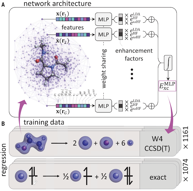
Part of Figure 1 from the paper. (c) 2021 The authors

This paper presents a new ML-exchange-correlation potential that gives improved results compared to state-of-the-art functionals, especially for barriers. Most importantly, it demonstrates the importance of including fractional charge and spin in the training set when developing new functionals. Fractional charge-systems help reduce the self-interaction error while fractional spin-systems supplies information about static correlation. For example, the current functional gives reasonable bond dissociation curves and future functionals of this kind may work considerably better on transition metal-containing systems with significant multi-reference character.   

This work is licensed under a Creative Commons Attribution 4.0 International License.

Quantum harmonic free energies for biomolecules and nanomaterials

Alec F. White,  Chenghan Li, and Garnet Kin-Lic Chan (2021)
Highlighted by Jan Jensen

Figure 2 from the paper. (c) The authors. Reproduced under the CC-BY license.

This paper describes a method by which the harmonic vibrational free energy contributions can be accurately approximated at roughly 10% of the cost of a conventional Hessian calculation.

The equations for the vibrational free energy contributions are recast in terms of the trace of a matrix function (remember that the trace of a matrix is equal to the sum of its eigenvalues). This removes the need for matrix diagonalisation, which is costly for large matrices. Then they use a stochastic estimator of the trace where the trace is rewritten in terms of displacements along $n$ random vectors. The accuracy of free energy differences can be further increased by using the same random vectors for both reactants and products.

The accuracy of this approximation increases with the number of displacement vectors (and, hence, gradient evaluations) used. The authors tested in one several large systems, such as protein-ligand binding,  and found that sub-kcal/mol accuracy can be obtained at about 10% of the cost of a conventional Hessian calculation plus diagonalisation.

It is now quite common to scale the entropy contributions from small (<100 cm$^{-1}$) frequencies to get better numerical stability. I am not sure whether this is possible in the current approach since individual frequencies are not computed explicitly.

The code and data is "available upon reasonable request" 😕

This work is licensed under a Creative Commons Attribution 4.0 International License.

Explaining and avoiding failures modes in goal-directed generation

Maxime Langevin, Rodolphe Vuilleumier, and Marc Bianciotto (2021) 
Highlighted by Jan Jensen

Figure 1 from the paper. (c) the authors 2021. Reproduced in the CC-BY-NC license

When you use search algorithms to optimise molecular properties predicted by ML-models, there is always the danger of going into regions of chemical space where the ML model no longer makes accurate predictions. Last year Renz et al. tried to quantify this phenomenon and basically concluded that it is a big problem. The current paper does not agree.

Renz et al. develop three different RF models as shown in the figure above for classifying bioactivity. In principle, all three models should give the same predictions. A search algorithm is then used to find molecules for which one of the models (the optimisation model) predict high scores, and these molecules are rescored using the other two control models. As the search proceed, these scores begin to diverge, leading Renz et al. to conclude that the search algorithms exploit biases particular to the optimisation model and does not, in fact, predict molecules that are truly active.

I almost highlighted this paper when it first appeared but was concerned by the relatively small sizes of the data sets used: 842, 667, and 842 molecules with 40, 140, and 59 active molecules, respectively. The paper by Langevin et al. suggests that this concern was justified.  

First they created a holdout set of 10% of the molecules, and repeated the procedure by Renz et al. on the remaining 90%. They showed that the difference in performance for the holdout set are the same as those observed by Renz et al, i.e. these differences have to do with the models/training sets themselves and not necessarily with the search algorithms. 

To show that it, in fact, has nothing to do with the search algorithms, they then demonstrated that the difference in model performance can be significantly reduced using two different approaches. One is to split the two data sets such that they are as similar as possible. Another is to use a better RF model: 200 trees and at least 3 samples per leaf, instead of 100 trees and 1 sample per leaf originally used by Renz et al.

This work is licensed under a Creative Commons Attribution 4.0 International License.

Benchmarking molecular feature attribution methods with activity cliffs

José Jiménez-Luna, Miha Skalic, and Nils Weskamp (2021)
Highlighted by Jan Jensen

Figure 1 from the paper. (c) The authors 2021. Reproduced under the CC-BY-NC license.

This is a follow-up of sorts on a previous post on trying to explain ML models using feature attribution.  While the idea is very attractive it is not obvious how to best benchmark such methods for chemical applications since it's rarely clear what the right answer is. Most benchmarking so far has therefore been done on toy problems that basically amount to substructure identification. 

This paper suggests that a solution to this is trying to identify activity cliffs in protein-ligand binding data, i.e. small structural changes that lead to large changes in binding affinity. The idea is that the atom attribution algorithms should identify these structural differences as illustrated in the figure above. The paper goes on to test this premise for an impressive number of feature attribution algorithms on an impressive number of datasets. 

The main conclusion is that none of the methods work unless the molecule pairs are included in the training set! Thus the authors ...

"... discourage the overall use of modern feature attribution methods in prospective lead optimization applications, and particularly those that work in combination with message-passing neural networks."

However, this paper by Cruz-Monteagudo et al. argues that ML models in general should fail to predict activity cliffs. One way to view activity cliffs is as exceptions that test the rules and ML models are supposed to learn the rules. The only way to predict the exceptions is to memorise them (i.e. overfit). 

On the other hand the examples shown above are, in my opinion, pretty drastic changes in structure that may not fit the conventional definition of activity cliffs and could conceivably be explained with learned rules. Clearly the feature attribution methods tested by Jiménez-Luna et al. are not up to the task. Or perhaps such methods require a larger training set to work. One key questions the authors didn't discuss is whether the ML models also fail to predict the change in binding affinity in addition to failing to correctly attribute the change.  



This work is licensed under a Creative Commons Attribution 4.0 International License.

Evidential Deep Learning for Guided Molecular Property Prediction and Discovery

Ava P. Soleimany, Alexander Amini, Samuel Goldman, Daniela Rus, Sangeeta N. Bhatia, and Connor W. Coley 2021
Highlighted by Jan Jensen

TOC figure from the paper. (c) 2021 The authors. Reproduced under the CC BY NC ND license

While knowing the uncertainty of a ML-predicted value is valuable, it is really only the Gaussian process method that delivers a rigorous estimate of this. If you want to use other ML methods such as NN you have to use more ad hoc methods like the ensemble or dropout methods and these only report of the uncertainty in the model parameters (if you retrain your model you'll get slightly different answers) and not on the uncertainty in the data (if you remeasure your data you'll get slightly different answers).

This paper presents a way to quantify both types of uncertainty for NN models (evidential learning). To apply it you change your output layer to output 4 values instead of 1 and you use a special loss function. One of the four output values is your prediction while the remaining 3 output values are plugged into a formula that gives you the uncertainty.

The paper compares this approach to the ensemble and dropout methods and shows that the evidential learning approach usually works better, i.e. there's a better correlation between the predicted uncertainty and the deviation from the ground truth. Note that it's a little tricky to quantify this correlation: if the error is random (which is the basic assumption behind all this) then the error can, by chance, be very small for a point with large uncertainty; it's just less likely compared to a point with low uncertainty. 

The code is available here (note the link in the paper is wrong)


This work is licensed under a Creative Commons Attribution 4.0 International License.

Interactions between large molecules pose a puzzle for reference quantum mechanical methods

Yasmine S. Al-Hamdani, Péter R. Nagy, Andrea Zen, Dennis Barton, Mihály Kállay, Jan Gerit Brandenburg and  Alexandre Tkatchenko (2021)
Highlighted by Jan Jensen

Figure 1 from the paper (c) The authors. Reproduced under the CC-BY licence

CCSD(T) and DMC are two gold-standard methods that should give the same results, and usually do. However, this study finds three systems for which the disagreement is unexpected large, up to 7.6 kcal/mol. It's not clear why and and it's not clear which method is correct. Since we use these methods to develop and benchmark other methods this is a real problem. 

Now, there could be many reasons for the discrepancy and the authors have considered all of them and discounted most of them. The remaining reasons, such as higher order terms in the CC expansion, are practically impossible to check at presents. It also hard to believe that they would make such a large contributions to the interaction energy of two closed shell systems. 

But there must be some reason for the discrepancy and when it is found we will most likely have learned something new about these methods.

This work is licensed under a Creative Commons Attribution 4.0 International License.

Bayesian optimization of nanoporous materials

Aryan Deshwal, Cory M. Simon, and Janardhan Rao Doppa (2021)
Highlighted by Jan Jensen

Figure 5 from the paper. (c) the authors. Reproduced under the CC-BY license.

This is another example of searching chemical space for systems with extreme property values by continuously updating a surrogate ML model of the property. I wrote about another such example, by Graff et al., here, but the main new thing here (IMO) is the low number of property evaluations needed to train the surrogate model.

The property of interest is the methane deliverable capacity (y) of covalent organic frameworks (COFs) which has been predicted by expensive MD calculations for ca 70,000 COFs. Ten randomly selected datapoints are used to train a Gaussian Process (GP) surrogate model. Bayesian optimisation (BO) is then used to identify the COF that is most likely to improve the surrogate model (based on the predicted y-value and the uncertainty of of the prediction), which is re-evaluated using MD. The MD value then added to the training set and the process is repeated for up to 500 steps. 

Already after 100 steps (110 MD evaluations including the initial training set), the best COF is identified as are 25% of the top-100 COFs, which is quite impressive. For comparison, the smallest training set in the previous study by Graff et al. is 100 and they need a training set of 300 to get to 25%. On the other hand, Graff et al. get up to ca 70% of the top 100 with a training set of 500, compared to ca 50% in this study (but the chemical space of Graff et al. is only 10,000 so it's a bit hard to compare).

The main lesson (IMO) is that's it's worth trying to start with very small training sets for these approaches.

This work is licensed under a Creative Commons Attribution 4.0 International License.

Using attribution to decode binding mechanism in neural network models for chemistry

Kevin McCloskey, Ankur Talya, Federico Montia, Michael P. Brennera, and Lucy J. Colwella (2019)
Highlighted by Jan Jensen

Part of Figure 3. Red indicates atoms that make positive contributions to the predicted values.

Copyright (2019) National Academy of Sciences.

This paper shows that state-of-the-art ML models can easily be fooled even for relatively trivial classification problems. 

The authors generate several synthetic classification sets using simple rules, such as the presence of a phenyl group, and train both a graph-convolutional and message passing NN. Not surprisingly, the hold-out performance is near perfect with AUCs near 1.000. 

Then they use a technique called integrated gradients to compute atomic contributions to the predictions and check whether these contributions match the rules used to create the data sets. For example, if the ground truth rule is the presence of a benzene ring, then only benzene ring atoms should make significant positive contributions. For some ground truth rules, this is often not the case!

Figure 3A above shows a case where the ground truth rule is the presence of three groups: a phenyl, a primary amine, and an ether. While this model is correctly classified there are significant atomic contributions from some of the fused ring atoms. So either the atomic contributions are mis-assigned by the integrated gradients method or the prediction is correct for the wrong reasons. The authors argue that it is the latter because three atomic changes in and near the fused ring (Figure 3B) results in a molecule that the model mis-classifies.

The authors note:

It is dangerous to trust a model whose predictions one does not understand. A serious issue with neural networks is that, although a held-out test set may suggest that the model has learned to predict perfectly, there is no guarantee that the predictions are made for the right reason. Biases in the training set can easily cause errors in the model’s logic. The solution to this conundrum is to take the model seriously: Analyze it, ask it why it makes the predictions that it does, and avoid relying solely on aggregate accuracy metrics.

The integrated gradient (IG) method is interesting in and of itself, so a few more words on that:

Jiménez-Luna et al. have since shown that the IG approach can be used to extract pharmacophores from models trained on experimental data sets. 

IG can only be applied to fully differentiable models such as NNs but Riniker and Landrum and Sheridan have developed fingerprint-based approaches that can be applied to any ML model but are theoretically more ad hoc. The Riniker-Landrum approach is available in RDKit while Jiménez-Luna et al. provide an implementation of the Sheridan approach, and also identify several examples where IG and the Sheridan approach gives different interpretations.

This work is licensed under a Creative Commons Attribution 4.0 International License.

ChemDyME: Kinetically Steered, Automated Mechanism Generation Through Combined Molecular Dynamics and Master Equation Calculations

Robin J. Shannon, Emilio Martínez-Núñez, Dmitrii V. Shalashilin, David R. Glowacki (2021)
Highlighted by Jan Jensen

Figure 1 from the paper (c) The authors 2021. Reproduced under the CC-BY license

ChemDyME couples metadynamics statistical  rate  theory to automatically find kinetically important reactions and then solve the time evolution of the species in the evolving network. 

There are three steps as shown in the figure above:

1. Molecular Dynamics (MD) where semiempirical metadynamics simulations are used to identify products that are likely to be connected to the reactant by low barriers. Specifically the boxed MD (BXD) metadynamics method where an extra term to the atomic velocities to steer the MD away from previously explored regions of configuration space. The MD stops when changes in atomic connectivity is detected.

2. Optimisation and Refinement (OR) where the products structures are optimised an the TSs to the reactant are located at a higher level of theory. The initial guess for the TS geometry is the first structure in the trajectory where the atomic connectivity changes. If that approach fails a spline-based reaction path method is used. The TSs are verified by IRCs.

3. Master Equation (ME) where the set of coupled kinetic equations are solved numerically. As the reaction network grows this can become computationally demanding, which is a problem when it is done on-the-fly. The authors therefore employ the Boxed Molecular Kinetics approach to speed things up.

These steps are then repeated using the kinetically most accessible product (identified by the ME step) as the reactant. The entire procedure is then repeated until a desired maximum reaction time is reached.

The authors test the procedure on two well studies systems and show that the procedure indeed identifies the most important reactions in the reaction network.

Disclaimer: My group has developed a similar approach for the first two steps.

This work is licensed under a Creative Commons Attribution 4.0 International License.

Leveraging Uncertainty in Machine Learning Accelerates Biological Discovery and Design

Brian Hie, Bryan D. Bryson, Bonnie Berger (2021)
Highlighted by Jan Jensen

Part of the TOC figure. (c) The authors. Reproduced under the CC-BY-NC-ND license

It is rare to see successful ML studies with training sets of 72 molecules, but this is one such study. 

The data set is 72 compounds with measured binding affinities to 442 different kinases, i.e. 32K datapoints. The Kds span a range of 0.1 nm to 10 μm. This data is used to train several ML models, some of which include uncertainty estimation and some which do not. The main finding is that for points with low uncertainties the ML model is better at separating active from inactive compounds. Interestingly, compounds with low uncertainty have extreme Kds.

The models (retrained on the whole dataset) is then used to screen a set of 10,833 purchasable compounds. The top five candidates for each model where purchased and checked against four different kinases (i.e. 20 ligand-kinase pairs per model). For the uncertainty based ML models the top candidates are molecules with both low Kd and low uncertainty, while for the other models the decision was made solely based on Kd.

None of the molecules picked solely based on Kd showed at Kd less than 10 μm, whereas 18, 10, and 2 ligand-kinase pairs had Kds lower than 10 μm, 100 nm, and 1 nm, respectively. 

Some ML details: The molecules where featurised using a graph convolutional junction tree approach (JTNN-VAE), which was found to work better han fingerprints (data not shown). The uncertainty is predicted using four different approaches: GP regression (GP), GP regression of the MLP error (MLP+GP), Bayesian multilayer perceptron (BMLP) and an ensemble of MLPs that each emits a Gaussian distribution (GMLPE). Nigam et al. recently published a very nice overview of such methods.

This work is licensed under a Creative Commons Attribution 4.0 International License.

Uncertainty Quantification Using Neural Networks for Molecular Property Prediction

Lior Hirschfeld, Kyle Swanson, Kevin Yang, Regina Barzilay, and Connor W. Coley 2020
Highlighted by Jan Jensen

Figure 3 from the paper. (c) American Chemical Society 2020

Given the blackbox nature of ML models it is very important to have some measure of how much to trust their predictions. There are many ways to do this paper shows "none of the methods we tested is unequivocally superior to all others, and none produces a particularly reliable ranking of errors across multiple data sets."

This conclusion is neatly summarised in the figure shown above for 5 common datasets, 2 different ML methods, and 4 different methods for uncertainty quantification. For each combination of these the plot shows the RMSE for for the 100, 50, 25, 10, and 5% of the test set on which the uncertainty quantification method calculated the lowest uncertainty for the hold-out set.

Generally, the RMSE drops as expected but the drops are in many cases decidedly modest past 50% and it can even increase in some cases. In most cases there is very little difference between the different uncertainty quantification methods, but sometimes there is and it's hard to predict when.

One thing that struck me when reading this paper is that many studies who include uncertainty quantification, e.g. using the ensemble approach, often just take it for granted that it works and don't present tests like this.

This work is licensed under a Creative Commons Attribution 4.0 International License.

Accelerating High-Throughput Virtual Screening Through Molecular Pool-Based Active Learning

David E. Graff, Eugene I. Shakhnovich, and Connor W. Coley (2020)
Highlighted by Jan Jensen

Figure 1 and part of Figure 2 from the paper. (c) The authors 2021. 

This paper shows how to find the highest scoring molecules in a very large library of molecules by scoring only a very small percentage of the library. The focus of the paper is docking scores but it can in principle to be used for any molecular property.

The general approach is simple: 

1. Start by picking a random sample of the library (say 100 molecules out of a library of 10.000 molecules) and evaluate their scores. 

2. Use these 100 points to train a machine-learning (ML) model to predict the scores.

3. Screen all 10,000 molecules using the ML model. The assumption is that training/using the ML model is much cheaper than evaluating the score.

4. Select the 100 best molecules according to the ML model, compute the scores, and use them to retrain the ML model.

5. Repeat steps 3 and 4.

The best molecules could be the best-scoring molecules (this a known as "greedy" optimisation). However, if the uncertainty of the ML prediction for each molecule can be quantified, there are several other options for what best is (use of these approaches are referred to as Bayesian optimisation).  The study investigates four selection functions involving standard deviations but finds the greedy approach works best.

The approach is tested on three different datasets with known docking scores of varying sizes (10K, 50K, 2M, and 99M). The study tests three different machine learning models: RF and NN using fingerprints as well as a graph convolutional model (which works best) and various choices batch sizes. 

In the case of the 99M dataset more than half of the top-50,000 scoring molecules can be found by docking only 600K molecules using this approach. 

However, let's turn that last sentence around: if you're developing an ML model to find high-scoring molecules your training set size needs to be 600K. Furthermore, the study shows that if you just pick 500K random molecules for your training set, your ML model won't identify any of the top-50,0000 molecules. You have to build this very large training set in this iterative fashion to get an ML model that can reliably identify the top-scoring molecules.

This work is licensed under a Creative Commons Attribution 4.0 International License.