Schrödinger-ANI: An Eight-Element Neural Network InteractionPotential with Greatly Expanded Coverage of Druglike Chemical Space

James M. Stevenson, Leif D. Jacobson, Yutong Zhao, Chuanjie Wu, Jon Maple, Karl Leswing, Edward Harder, and Robert Abel (2019)
Highlighted by Jan Jensen

There are a lot of ML models trained on HCNO data sets. This is fine for proof-of-concept, but severely limits applications to real world problems. For example HCNO-only molecules comprise only 46% of molecules in the CHEMBL database of drug-like molecules.

The main problem with extending these methods to other elements is that the size of the chemical space grows non-linearly with respect to the number of different elements. Furthermore, there aren't any generally available and comprehensive sets of molecules similar to QMx or GDB-x.

The current study extends the ANI-1 method to H, C, N, O, S, F, Cl, and P, which covers 94% of CHEMBL. The authors use a combination of stochastic sampling and extensive pre-screening to distill the training/validation set to only 10 million DFT single point calculations on relatively small molecules, which took "just a few days and at a very reasonable compute cost".

The main focus was on relative conformer energies, since the bulk of CPU time for many studies is typically spent on conformational searches. The RMSE for this data is 0.70 kcal/mol relative to DFT, which is quite impressive.

As the name suggests, the work was done at Schrödinger, so the method is not open sourced. However, an earlier version for 4 elements is available here. More importantly, the methodology behind the dataset generation is well described and appears to be practically feasible for academic labs.


This work is licensed under a Creative Commons Attribution 4.0 International License.

Unifying machine learning and quantum chemistry with a deep neural network for molecular wavefunctions

K. T. Schütt, M. Gastegger, A. Tkatchenko, K.-R. Müller & R. J. Maurer  (2019)

Highlighted by Jan Jensen

Figure 2 from the paper. © The Authors 2019. Reproduced under the CC-BY license.

This paper had received a lot of attention, so I had to see what the fuzz was about. The method (SchNOrb) uses a deep neural network to create a Hamiltonian matrix from 3D coordinates, which can then be diagonalised to yield orbital energies and orbitals. SchNOrb is trained to reproduce Hamiltonian and overlap matrix elements, total energies (which are computed as the sum of orbital energies in the ML model), and gradients all taken from AIMD trajectories. 

So it's a bit like the ANI-1 method except that you also get orbitals, which can be used to compute other properties without additional parameterisation. One crucial difference though is that, as far as I can tell, SchNOrb is parameterised for each molecule separately. 

The model uses about 93 million parameters for a >100 AO Hamiltonian and requires 25,000 structures and 80 GPU hours to train. Once trained it can predict an energy with meV accuracy in about 50 ms on a GPU.

The software is "available upon request".

The reviews are made available, and well worth reading.

This work is licensed under a Creative Commons Attribution 4.0 International License.

The minimum parameterization of the wave function for the many-body electronic Schrödinger equation. I. Theory and ansatz

Lasse Kragh Sørensen (2019)
Highlighted by Jan Jensen

It is well known that Full CI (FCI) scales exponentially with the basis set size. However, Sørensen claims that the "whole notion of the exponentially scaling nature of quantum mechanics simply stems from expanding the wavefunction in a sub-optimal basis",  i.e. one-electron functions. Sørensen goes on to argue that of two-ele tron functions (geminals) are used instead, the scaling is reduced to m(m−1)/2 where m is the number of basis functions.  Furthermore, because "the number of parameters is independent of the electronic structure the multi-configurational problem is a mere phantom summoned by a poor choice of basis for the wave function". 

I don't have the background to tell whether the arguments in this paper are correct and the main point os this post is to see if I can get some feedback from people who do have the background. 

In principle one could simply compare the new approach to FCI calculations but the new method isn't quite there yet:

A straight forward minimization of Eq. 84 unfortunately gives the solution for the two-electron problem of a +(N−2) charged system N/2 times so additional constraints must be introduced. These constraints can be found by the property of the wave function in limiting cases. The problem of finding the constraints for the geminals in the AGP ansatz is therefore closely related to finding the N-representability constraints for the two-body reduced density matrix (2-RDM). For the N-representability Mazziotti have showed a constructive solution[74] though the exact conditions are still illusive.[75, 76]  

This work is licensed under a Creative Commons Attribution 4.0 International License.

Boltzmann generators: Sampling equilibrium states of many-body systems with deep learning

Frank Noé, Simon Olsson, Jonas Köhler, Hao Wu (2019)
Highlighted by Jan Jensen

Figure 1A from the paper (Copyright © 2019 The Authors, some rights reserved)

The paper presents a novel method to predict free energy differences much more efficiently.  Currently, this is usually done by MD simulations and observing how often each state is visited along the trajectory. However, transitions between each state are rare, which means very long and costly trajectories, even when using various tricks to force the transitions.

The solution Noé et al. present is to "train a deep invertible neural network to learn a coordinate transformation from x to a so-called “latent” representation z, in which the low-energy configurations of different states are close to each other and can be easily sampled."

For example, the user supplies a few examples of each state [p_x(x)] and trains the NN to find a new set of variables (z) with a much simpler probability distribution [p_z(z)], by minimising the difference using the Kullback-Leibler divergence as a loss function.

Since the NN is invertible, one can now sample repeatedly from p_z(z) to get a more accurate p_x(x), which can then be reweighed to give the Boltzmann distribution. Since p_z(z) is a simple Gaussian most of the sampled structure will have a high Boltzmann probability, so you don't have to sample that many structures.

The technical main advance is the use of an invertible NN, that allow you to go both from x to z and z to x. This is done by using a NN architecture where only simple mathematically operations (addition and multiplication) that can be reversed (subtraction and division) are allowed.

It would be very interesting to see if a similar approach can be used for inverse design.


This work is licensed under a Creative Commons Attribution 4.0 International License.

Deflate to Understand Complex Molecular Kinetics

Brooke E. Husic & Frank Noé. arXiv: 1907.04101

Contributed by Jesper Madsen

Dimensionality reduction is at the core of understanding and making intuitive sense of complex dynamic phenomena in chemistry.  It is usually assumed that the slowest mode is the one of primary interest; however, it is critical to realize that this is not always so! A conceptual example hereof is a protein folding simulation (Lindorff-Larsen et al. Science 334, 517-520, 2011) where the slowest dynamical mode is not the folding itself (see Figure). What is the influence, then, of “non-slowest” modes in this process and how can it most appropriately be elucidated?

FIG: Figure 2 from the preprint: "(A) Sampled villin structures from the MD trajectory analyzed. Helical secondary structure is colored and coils are white. Each image represents five structures sampled from similar locations in TIC space as determined by a 250-center k-means model built upon the first three original TICs. The purple structure represents the folded state, and the blue structure represents the denatured state. The green structure is a rare helical misfolded state that we assert is an artifact. (B) Two-dimensional histograms for TICA transformations constructed from villin contact distances. Dashed lines indicate the regions corresponding to the sampled structures of the same color. The first TIC tracks the conversion to and from the rare artifact only. The second TIC tracks the majority of the folding process and correlates well with RMSD to the folded structure."

This work by Husic and Noé show how deflation can provide an answer to these questions. Technically speaking deflation is a collection of methods for how to modify a matrix after the largest eigenvalue is known in order to find the rest. In their provided example of the folding simulation, the dominant Time-lagged Independent Component (TIC) encapsulates the "artifact" variation that we are not really interested in. Thus, a constructed kinetic (Markov-state) model will be contaminated in several undesirable ways as discussed by the authors in great detail.  

In principle, this should be a very common problem since chemical systems have complex Hamiltonians. Perhaps the reason why we don’t see it discussed more is that ultra-rare events – real or artifact – may not usually be sampled during conventional simulations. So, with the increasing computational power available to us, and simulations approaching ever-longer timescales, this is likely something that we need to be able to handle. This preprint describes well how one can think about attacking these potential difficulties.   

Physical machine learning outperforms "human learning" in Quantum Chemistry

Anton V. Sinitskiy and Vijay S. Pande (2019)

Highlighted by Jan Jensen

Figure 1 from the paper

The paper presents a method to estimate DFT or CCSD(T) energies (computed using large basis sets) based only on HF/cc-pVDZ densities and energies. In order to avoid overfitting, the method must also estimate the corresponding DFT or CCSD densities. The method is trained and validated on a subset of the QM9 data set (i.e. on relative small molecules). It is first trained on DFT data (using 89K molecules) and then retrained on CC data for a smaller subset (3.6K molecules), both being subsets of the QM9 data set (i.e. relatively small molecules). The input density is evaluated in a 3D grid that is big enough to accommodate the largest molecule in the data set, so a new model would have to be trained for significantly larger molecules.

This “physical machine learning in Quantum Chemistry” (PML-QC) model reaches a mean absolute error in energies of molecules with up to eight non-hydrogen atoms as low as 0.9 kcal/mol relative to CCSD(T) values, which is quite impressive. In fact the authors speculate that 

With ML, it may become not required that an accurate quantum chemical method works fast enough for every new molecule that an end user may be interested in. Instead, the focus shifts to generating highly accurate results only for a finite dataset to be used for training, while the efficiency in practical applications is to be achieved via improvements in DNNs to make them faster and more accurate.

Much will depend how much the number of outliers can be reduced. For example, for PML-QC_DFT ca 5% of molecules have errors greater than 2.6 kcal/mol and this effect can be magnified for relative energies if the individual errors have opposite sign.

This work is licensed under a Creative Commons Attribution 4.0 International License.

Popular Integration Grids Can Result in Large Errors in DFT-Computed Free Energies

Andrea N. Bootsma and Steven E. Wheeler (2019)

Highlighted by Jan Jensen

 Figure 1B from the paper (CC BY-NC-ND 4.0)

 This paper has already been highlighted here and here, so I'll just briefly summarise.

The grid used for the numerical integration in DFT calculations is defined relative to the Cartesian axes, so rotating the molecule will change the integration grid and, hence, the energy. This has been known for some time and, f.eks. Gaussian09 uses a default grid size (Fine, 75,302) where the effect on the electronic energy variation is usually negligible.

Bootsma and Wheeler show that the vibrational entropy and, hence, the free energy is significantly more sensitive to grid size than the electronic energy. Using the Fine grid, the differences in relative free energy changes can be as large as 4 kcal/mol, which could significantly change conclusion regarding mechanisms, etc. The effect comes from the variation in low frequency vibrational modes and the effect can be reduced a little by scaling these frequencies. 

However, the errors really only become acceptable when using the UltraFine grid size, which is the default in Gaussian16, especially combined with frequency scaling (which one should do anyway to get consistent results). If you are using Gaussian09 or some other quantum program to compute relative free energies it is definitely a good idea to look at the default grid size and perform some tests.

Note that if you want to perform such tests yourself, you need to re-optimise the molecule after you rotate it because the gradient is also affected by the rotation.

This work is licensed under a Creative Commons Attribution 4.0 International License.

Combining the Power of J Coupling and DP4 Analysis on Stereochemical Assignments: The J-DP4 Methods

Grimblat, N.; Gavín, J. A.; Hernández Daranas, A.; Sarotti, A. M., Org. Letters 2019, 21, 4003-4007

Contributed by Steven Bachrach
Reposted from Computational Organic Chemistry with permission

I have written quite a number of posts on using quantum mechanics computations to predict NMR spectra that can aid in identifying chemical structure. Perhaps the most robust technique is Goodman’s DP4 method (post), which has seen some recent revisions (updated DP4, DP4+). I have also posted on the use of computed coupling constants (posts).

Grimblat, Gavín, Daranas and Sarotti have now combined these two approaches, using computed ¹H and ¹³C chemical shifts and ³J_HH coupling constants with the DP4 framework to predict chemical structure.¹

They describe two different approaches to incorporate coupling constants:

• dJ-DP4 (direct method) incorporates the coupling constants into a new probability function, using the coupling constants in an analogous way as chemical shifts. This requires explicit computation of all chemical shifts and ³J_HH coupling constants for all low-energy conformations.
• iJ-DP4 (indirect method) uses the experimental coupling constants to set conformational constraints thereby reducing the number of total conformations that need be sampled. Thus, large values of the coupling constant (³J_HH > 8 Hz) selects conformations with coplanar hydrogens, while small values (³J_HH < 4 Hz) selects conformations with perpendicular hydrogens. Other values are ignored. Typically, only one or two coupling constants are used to select the viable conformations.

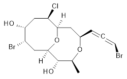
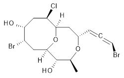
The authors test these two variants on 69 molecules. The original DP4 method predicted the correct stereoisomer for 75% of the examples, while dJ-DP4 correct identifies 96% of the cases. As a test of the indirect method, they examined marilzabicycloallenes A and B (1 and 2). DP4 predicts the correct stereoisomer with only 3.1% (1) or <0.1% (2) probability. dJ-DP4 predicts the correct isomer for 1 with 99.9% probability and 97.6% probability for 2. The advantage of iJ-DP4 is that using one coupling constant reduces the number of conformations that must be computed by 84%, yet maintains a probability of getting the correct assignment at 99.2% or better. Using two coupling constants to constrain conformations means that only 7% of all of the conformations need to be samples, and the predictive power is maintained.

1

2

Both of these new methods clearly deserve further application.

References

1. Grimblat, N.; Gavín, J. A.; Hernández Daranas, A.; Sarotti, A. M., “Combining the Power of J Coupling and DP4 Analysis on Stereochemical Assignments: The J-DP4 Methods.” Org. Letters 2019, 21, 4003-4007, DOI: 10.1021/acs.orglett.9b01193.

InChIs

1: InChI=1S/C15H21Br2ClO4/c1-8-15(20)14-6-10(17)12(19)7-11(18)13(22-14)5-9(21-8)3-2-4-16/h3-4,8-15,19-20H,5-7H2,1H3/t2-,8-,9+,10-,11+,12+,13+,14+,15-/m0/s1
InChIKey=APNVVMOUATXTFG-NTSAAJDMSA-N

2: InChI=1S/C15H21Br2ClO4/c1-8-15(20)14-6-10(17)12(19)7-11(18)13(22-14)5-9(21-8)3-2-4-16/h3-4,8-15,19-20H,5-7H2,1H3/t2-,8-,9-,10-,11+,12+,13+,14+,15-/m0/s1
InChIKey=APNVVMOUATXTFG-SSBNIETDSA-N

'
This work is licensed under a Creative Commons Attribution-NoDerivs 3.0 Unported License.

The logic of translating chemical knowledge into machine-processable forms: A modern playground for physical-organic chemistry

Karol Molga, Ewa P. Gajewska, Sara Szymkuć, and Bartosz A. Grzybowski (2019)

Highlighted by Jan Jensen

Figure 11 from the paper (c) RSC

This paper offers a, to me, fascinating "look behind the scenes" of Chematica. At the core this program has 75,000 handcrafted reaction rules (SMARTS and Reaction SMARTS strings as shown in the above figure) extracted from the literature (which took over a decade). The authors estimate that there ca 3000-5000 new reaction classes/types appearing in the literature each years and "that there are on the order of 100,000 distinct reaction classes constituting the body of modern organic chemistry. So their work is almost done :).

The paper does a really excellent job of outlining the challenges involved in constructing these rules and present several cases where the rules must be augmented by ML, MM, and Hückel calculations in order to take non-local structural (e.g. strain and steric hindrance) and electronic effects (e.g. on regioselectivity) into account. Such calculations must be done on the millisecond time scale as many thousand intermediates must be inspected during a retrosynthetic search. At the same time they must be very accurate as inaccuracies accumulate with each step on the retrosynthetic path.

It will be very interesting to see if purely ML-based alternatives can beat this approach!


This work is licensed under a Creative Commons Attribution 4.0 International License.

Vibrational Signatures of Chirality Recognition Between α-Pinene and Alcohols for Theory Benchmarking

Medel, R.; Stelbrink, C.; Suhm, M. A., Angew. Chem. Int. Ed. 2019, 58, 8177
Contributed by Steven Bachrach
Reposted from Computational Organic Chemistry with permission

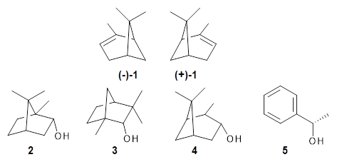
Can vibrational spectroscopy be used to identify stereoisomers? Medel, Stelbrink, and Suhm have examined the vibrational spectra of (+)- and (-)-α-pinene, (±)-1, in the presence of four different chiral terpenes 2-5.¹ They recorded gas phase spectra by thermal expansion of a chiral α-pinene with each chiral terpene.

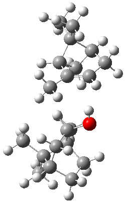
For the complex of 4 with (+)-1 or (-)-1 and 5 with (+)-1 or (-)-1, the OH vibrational frequency is identical for the two different stereoisomers. However, the OH vibrational frequencies differ by 2 cm^-1 with 3, and the complex of 3/(+)-1 displays two different OH stretches that differ by 11 cm^-1. And in the case of the complex of α-pinene with 2, the OH vibrational frequencies of the two different stereoisomers differ by 11 cm^-1!

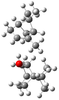
The B3LYP-D3(BJ)/def2-TZVP optimized geometry of the 2/(+)-1 and 2/(-)-1 complexes are shown in Figure 2, and some subtle differences in sterics and dispersion give rise to the different vibrational frequencies.

2/(+)-1

2/(-)-1

Figure 2. B3LYP-D3(BJ)/def2-TZVP optimized geometry of the 2/(+)-1 and 2/(-)-1

Of interest to readers of this blog will be the DFT study of these complexes. The authors used three different well-known methods – B3LYP-D3(BJ)/def2-TZVP, M06-2x/def2-TZVP, and ωB97X-D/def2-TZVP – to compute structures and (most importantly) predict the vibrational frequencies. Interestingly, M06-2x/def2-TZVP and ωB97X-D/ def2-TZVP both failed to predict the vibrational frequency difference between the complexes with the two stereoisomers of α-pinene. However, B3LYP-D3(BJ)/def2-TZVP performed extremely well, with a mean average error (MAE) of only 1.9 cm^-1 for the four different terpenes. Using this functional and the larger may-cc-pvtz basis set reduced the MAE to 1.5 cm^-1 with the largest error of only 2.5 cm^-1.

As the authors note, these complexes provide some fertile ground for further experimental and computational study and benchmarking.

Reference

1. Medel, R.; Stelbrink, C.; Suhm, M. A., “Vibrational Signatures of Chirality Recognition Between α-Pinene and Alcohols for Theory Benchmarking.” Angew. Chem. Int. Ed. 2019, 58, 8177-8181, DOI: 10.1002/anie.201901687.

InChIs

(-)-1, (-)-α-pinene: InChI=1S/C10H16/c1-7-4-5-8-6-9(7)10(8,2)3/h4,8-9H,5-6H2,1-3H3/t8-,9-/m0/s1
InChIKey=GRWFGVWFFZKLTI-IUCAKERBSA-N

(+)-1, (-)-α-pinene: InChI=1S/C10H16/c1-7-4-5-8-6-9(7)10(8,2)3/h4,8-9H,5-6H2,1-3H3/t8-,9-/m1/s1
InChIKey=GRWFGVWFFZKLTI-RKDXNWHRSA-N

2, (-)borneol: InChI=1S/C10H18O/c1-9(2)7-4-5-10(9,3)8(11)6-7/h7-8,11H,4-6H2,1-3H3/t7-,8+,10+/m0/s1
InChiKey=DTGKSKDOIYIVQL-QXFUBDJGSA-N

3, (+)-fenchol: InChI=1S/C10H18O/c1-9(2)7-4-5-10(3,6-7)8(9)11/h7-8,11H,4-6H2,1-3H3/t7-,8-,10+/m0/s1
InChIKey=IAIHUHQCLTYTSF-OYNCUSHFSA-N

4, (-1)-isopinocampheol: InChI=1S/C10H18O/c1-6-8-4-7(5-9(6)11)10(8,2)3/h6-9,11H,4-5H2,1-3H3/t6-,7+,8-,9-/m1/s1
InChIKey=REPVLJRCJUVQFA-BZNPZCIMSA-N

5, (1S)-1-phenylethanol: InChI=1S/C8H10O/c1-7(9)8-5-3-2-4-6-8/h2-7,9H,1H3/t7-/m0/s1
InChIKey=WAPNOHKVXSQRPX-ZETCQYMHSA-N

'
This work is licensed under a Creative Commons Attribution-NoDerivs 3.0 Unported License.

Activity-Based Screening of Homogeneous Catalysts through the Rapid Assessment of Theoretically Derived Turnover Frequencies

Matthew D. Wodrich, Boodsarin Sawatlon, Ephrath Solel, Sebastian Kozuch, and Clémence Corminboeuf (2019)
Highlighted by Jan Jensen

Figure 1. Adapted from images in the preprint posted under the CC-BY-NC-ND 4.0 license

This paper combines Corminboufs' work on linear free energy scaling relationships (LFESR) and volcano plots in homogeneous catalysis with Kozuch and Shaik's energy span model. 

LFESRs linearly relate the reaction energies of barrier heights to a single reaction energy. In this work the all the barriers and reaction energies in Figure 1a is computed via the free energy difference between 1 and 4 [ΔG(4)]

The volcano plot is then obtained by plotting the largest free energy difference in the cycle as a function of ΔG(4). In this particular case that is the barrier between 1 and 4 when ΔG(4) is small and the energy difference between 2 and 3 when  ΔG(4) is large. The optimum catalysts is the one with a ΔG(4) for which these two lines meet and one can screen for such catalyst by computing a single free energy difference.

One problem with thus approach is that the largest free energy difference in the cycle is not always directly related to the turn over frequency (TOF), which is what is measured experimentally. In principle, the TOF should be determined by microkinetic modeling for each value of ΔG(4) to find the maximum TOF. But in this work TOFs are efficiently estimated by the energy span model, which basically considers all energy differences in the cycle (e.g. also between 1 and 3).

Using the TOF plot different energy differences between important and the optimum ΔG(4) value decreases (Figure 1b). The points in Figure 1b show the corresponding TOFs computed without the LFESRs and demonstrate the accuracy of this approach.

This work is licensed under a Creative Commons Attribution 4.0 International License.

Exploration of Chemical Compound, Conformer, and Reaction Space with Meta-Dynamics Simulations Based on Tight-Binding Quantum Chemical Calculations

S. Grimme (2019)

Highlighted by Jan Jensen

The paper describes a new way to search for conformers, chemical reactions, and estimate barriers using the semiempirical GFNn-XTB method using meta-dynamics. A force term is included that scales exponentially with the Cartesian RMSD from previously found structures, thereby forcing the MD explore new areas of phase space. For simulations with more than one molecule it is necessary to add a constraining potential so that the RMSD cannot be increased simply by increasing the distance between molecules. Each individual MD can be relatively short and most of the CPU time is actually spend on energy minimising the snapshots that are saved.

The results depend on a few hyperparameters, so several MD simulations with different values are run in parallel. Because of the extra force the temperature is also a hyperparameters so the method doesn't necessarily tell you what reactions are most likely to occur at, say, 300K.

The conformational search is tested on 22 (mostly) organic molecules and includes the GFN2-xTB energies of the lowest energy conformer for each molecules. This is a valuable benchmark set for other conformational search algorithms designed to find the global minimum.

This work is licensed under a Creative Commons Attribution 4.0 International License.

Ambimodal Trispericyclic Transition State and Dynamic Control of Periselectivity

Xue, X.-S.; Jamieson, C. S.; Garcia-Borràs, M.; Dong, X.; Yang, Z.; Houk, K. N., J. Am. Chem. Soc. 2019, 141, 1217
Contributed by Steven Bachrach
Reposted from Computational Organic Chemistry with permission

A major topic of this blog has been the growing body of studies that demonstrate that dynamic effects can control reaction products (see these posts). Often these examples crop up with valley ridge inflection points. Another cause can be bispericyclic transition states, first discovered by Caramello et al for the dimerization of cyclopentadiene.¹ The Houk group now reports on the first trispericyclic transition state.²

Using ωB97X-D/6-31G(d), they examined the reaction of the tropone derivative 1 with dimethylfulvene 2. Three possible products can arrive from different pericyclic reactions: 3, the [4+6] product; 4, the [6+4] product; and 5, the [8+2] product. The thermodynamic product is predicted to be 5, but it is only 1.2 kcal mol^-1 lower in energy than 4 and 6.2 kcal mol^-1 lower than 3.

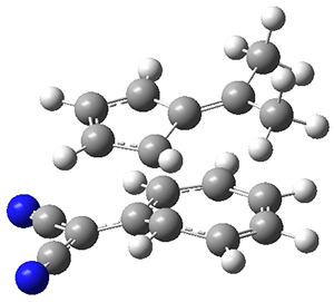
They identified one transition state originating from the reactants TS1. Hypothesizing that it would be trispericyclic, they performed a molecular dynamics study with trajectories starting from TS1. They ran a total of 142 trajectories, and 87% led to 3, 3% led to 4, and 3% led to 5. This demonstrates the unusual nature of TS1 and the dynamic effects on this reaction surface.

TS1
TS2	TS3

Figure 1. ωB97X-D/6-31G(d) optimized geometries of TS1-TS3.

Additionally, there are two different Cope rearrangements (through TS2 and TS3) that convert 3 into 4 and 5. Some trajectories can pass from TS1 and then directly through either TS2 or TS3 and these give rise to products 4 and 5. In other words, some trajectories will pass from a trispericyclic transition state and then through a bispericyclic transition state before ending in product.

References

1. Caramella, P.; Quadrelli, P.; Toma, L., “An Unexpected Bispericyclic Transition Structure Leading to 4+2 and 2+4 Cycloadducts in the Endo Dimerization of Cyclopentadiene.” J. Am. Chem. Soc. 2002, 124, 1130-1131, DOI: 10.1021/ja016622h

2. Xue, X.-S.; Jamieson, C. S.; Garcia-Borràs, M.; Dong, X.; Yang, Z.; Houk, K. N., “Ambimodal Trispericyclic Transition State and Dynamic Control of Periselectivity.” J. Am. Chem. Soc. 2019, 141, 1217-1221, DOI: 10.1021/jacs.8b12674.

InChIs

1: InChI=1S/C10H6N2/c11-7-10(8-12)9-5-3-1-2-4-6-9/h1-6H
InChIKey=KAWLLELUFONBGI-UHFFFAOYSA-N

2: InChI=1S/C8H10/c1-7(2)8-5-3-4-6-8/h3-6H,1-2H3
InChIKey=WXACXMWYHXOSIX-UHFFFAOYSA-N

3: InChI=1S/C18H16N2/c1-11(2)17-15-7-8-16(17)14-6-4-3-5-13(15)18(14)12(9-19)10-20/h3-8,13-16H,1-2H3
InChIKey=DRPXVBLNTKGMTB-UHFFFAOYSA-N

4: InChI=1S/C18H16N2/c1-18(2)13-6-8-14(12(10-19)11-20)15(9-7-13)16-4-3-5-17(16)18/h3-9,13,15-16H,1-2H3
InChIKey=FSIPGNLAWKVXDD-UHFFFAOYSA-N

5: InChI=1S/C18H16N2/c1-12(2)13-8-9-16-17(13)14-6-4-3-5-7-15(14)18(16,10-19)11-20/h3-9,14,16-17H,1-2H3/t14?,16-,17-/m1/s1
InChIKey=SYLWEGLODFLARZ-VNCLPFQGSA-N

'
This work is licensed under a Creative Commons Attribution-NoDerivs 3.0 Unported License.

A Universal Density Matrix Functional from Molecular Orbital-Based Machine Learning: Transferability across Organic Molecules

Lixue Cheng, Matthew Welborn, Anders S. Christensen, and Thomas F. Miller III

Highlighted by Jan Jensen

Figure 3c from the paper, showing results for MP2 correlation energies

Some years ago I wrote about the ∆-ML approach where ML is used to estimate the energy difference between expensive and cheap methods based on the molecular structure. I remember wondering at the time whether additional information could be extracted from the cheap method and used as descriptors. 

This has now been tested for correlation energies and it does indeed lead to a significant improvement in accuracy. The method uses Fock, Coulomb, and exchange matrix elements in an LMO basis (which makes me wonder why it's called a density matrix functional) and Gaussian process regression (GPR) to machine learn the LMO contributions to MP2, CCSD, and CCSD(T) correlation energies.

Using just 140 molecules with 7 heavy atoms the MOB-ML method can be trained to give reasonably accurate results for molecules with 13 heavy atoms (see figure above), and offer a significant improvement over the ∆-ML approach. An MAE of 0.25 mH/heavy atom translates into an MAE of roughly 2 kcal/mol for a molecule with 13 heavy atoms, which can translate into 4 kcal/mol ∆E-errors depending on the sign, so the method may not be quite accurate enough for many purposes yet. Unfortunately, it doesn't look like training on more molecules leads to additional improvements for transferability to larger molecules, but this is definitely a promising step in the right direction.

This work is licensed under a Creative Commons Attribution 4.0 International License.

Planar rings in nano-Saturns and related complexes

Bachrach, S. M., Chem. Commun. 2019, 55, 3650-3653

Contributed by Steven Bacharach
Reposted from Computational Organic Chemistry with permission

For the past twelve years, I have avoided posting on any of my own papers, but I will stoop to some shameless promotion to mention my latest paper,¹ since it touches on some themes I have discussed in the past.

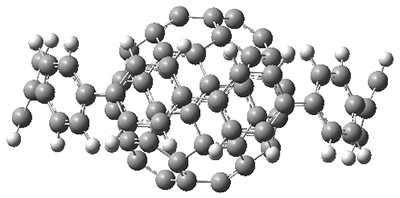
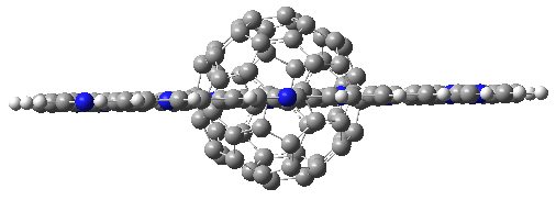
Back in 2011, Iwamoto, et al. prepared the complex of C₆₀ 1 surrounded by [10]cycloparaphenylene 2 to make the Saturn-like system 3.² Just last year, Yamamoto, et al prepared the Nano-Saturn 5a as the complex of 1 with the macrocycle 4a.³ The principle idea driving their synthesis was to utilize a ring that is flatter than 2. The structures of 3 and 5b (made with the parent macrocycle 4b) are shown in side view in Figure 1, and clearly seen is the achievement of the flatter ring.

3

5b

7

Figure 1. Computed structures of 3, 5, and 7.

However, the encompassing ring is not flat, with dihedral angles between the anthrenyl groups of 35°. This twisting is due to the steric interactions of the ortho-ortho’ hydrogens. A few years ago, my undergraduate student David Stück and I suggested that selective substitution of a nitrogen for one of the C-H groups would remove the steric interaction,⁴ leading to a planar poly-aryl system, such as making twisted biphenyl into the planar 2-(2-pyridyl)-pyridine (Scheme 1)

Scheme 1.

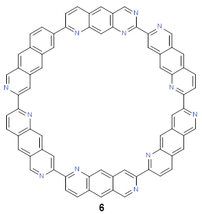
Following this idea leads to four symmetrical nitrogen-substituted analogues of 4b; and I’ll mention just one of them here, 6.

As expected, 6 is perfectly flat. The ring remains flat even when complexed with 1 (as per B3LYP-D3(BJ)/6-31G(d) computations), see the structure of 7 in Figure 1.

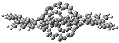
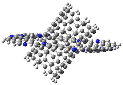
I also examined the complex of the flat macrocycle 6 (and its isomers) with a [5,5]-nanotube, 7. The tube bends over to create better dispersion interaction with the ring, which also become somewhat non-planar to accommodate the tube. Though not mentioned in the paper, I like to refer to 7 as Beyoncene, in tribute to All the Single Ladies.

Figure 2. Computed structure of 7.

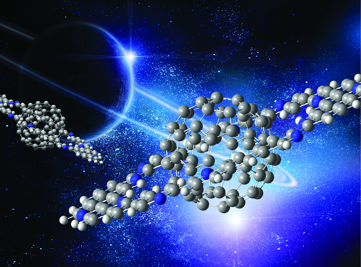
My sister is a graphic designer and she made this terrific image for this work:

References

1. Bachrach, S. M., “Planar rings in nano-Saturns and related complexes.” Chem. Commun. 2019, 55, 3650-3653, DOI: 10.1039/C9CC01234F.

2. Iwamoto, T.; Watanabe, Y.; Sadahiro, T.; Haino, T.; Yamago, S., “Size-Selective Encapsulation of C₆₀ by [10]Cycloparaphenylene: Formation of the Shortest Fullerene-Peapod.” Angew. Chem. Int. Ed. 2011, 50, 8342-8344, DOI: 10.1002/anie.201102302

3. Yamamoto, Y.; Tsurumaki, E.; Wakamatsu, K.; Toyota, S., “Nano-Saturn: Experimental Evidence of Complex Formation of an Anthracene Cyclic Ring with C60.” Angew. Chem. Int. Ed. 2018 , 57, 8199-8202, DOI: 10.1002/anie.201804430.

4. Bachrach, S. M.; Stück, D., “DFT Study of Cycloparaphenylenes and Heteroatom-Substituted Nanohoops.” J. Org. Chem. 2010, 75, 6595-6604, DOI: 10.1021/jo101371m

InChIs

4b: InChI=1S/C84H48/c1-13-61-25-62-15-3-51-33-75(62)43-73(61)31-49(1)50-2-14-63-26-64-16-4-52(34-76(64)44-74(63)32-50)54-6-18-66-28-68-20-8-56(38-80(68)46-78(66)36-54)58-10-22-70-30-72-24-12-60(42-84(72)48-82(70)40-58)59-11-23-71-29-69-21-9-57(39-81(69)47-83(71)41-59)55-7-19-67-27-65-17-5-53(51)35-77(65)45-79(67)37-55/h1-48H
InChIKey=ZYXXLAYETADMDM-UHFFFAOYSA-N

6: InChI=1S/C72H36N12/c1-2-38-14-44-20-45-25-67(73-31-50(45)13-37(1)44)57-9-4-39-15-51-32-74-68(26-46(51)21-61(39)80-57)58-10-5-40-16-52-33-75-69(27-47(52)22-62(40)81-58)59-11-6-41-17-53-34-76-70(28-48(53)23-63(41)82-59)60-12-7-42-18-54-35-77-71(29-49(54)24-64(42)83-60)72-78-36-55-19-43-3-8-56(38)79-65(43)30-66(55)84-72/h1-36H
InChIKey=NSSCKPFBHGOOIJ-UHFFFAOYSA-N

'
This work is licensed under a Creative Commons Attribution-NoDerivs 3.0 Unported License.